- Catalogs
- Dantec Dynamics
- Constant Temperature Anemometry
Constant Temperature Anemometry
1 /1Page
Constant Temperature Anemometry
1 /1Page
Catalog excerpts
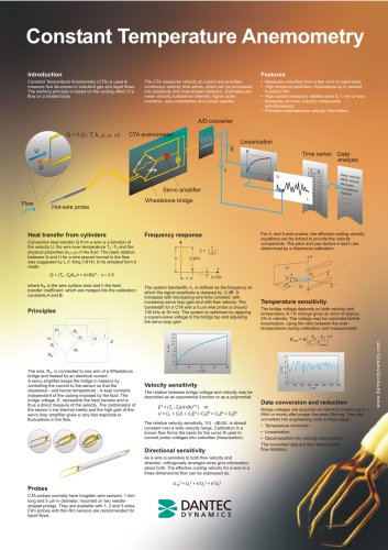
Introduction Constant Temperature Anemometry (CTA) is used to measure fine structures in turbulent gas and liquid flows. The working principle is based on the cooling effect of a flow on a heated body. The CTA measures velocity at a point and provides continuous velocity time series, which can be processed into amplitude and time-domain statistics. Examples are mean velocity, turbulence intensity, higher order moments, auto-correlations and power spectra. Measures velocities from a few cm/s to supersonic High temporal resolution: fluctuations up to several hundred kHz High spatial resolution: eddies down to 1 mm or less Measures all three velocity components simultaneously Heat transfer from cylinders Convective heat transfer Q from a wire is a function of the velocity U, the wire over-temperature Tw -To and the physical properties (k,p,ji) of the fluid. The basic relation between Q and U for a wire placed normal to the flow was suggested by L.V. King (1914). In its simplest form it reads: where Aw is the wire surface area and h the heat transfer coefficient, which are merged into the calibration constants A and B. The wire, Rw, is connected to one arm of a Wheatstone bridge and heated by an electrical current. A servo amplifier keeps the bridge in balance by controlling the current to the sensor so that the resistance - and hence temperature - is kept constant, independent of the cooling imposed by the fluid. The bridge voltage, E, represents the heat transfer and is thus a direct measure of the velocity. The combination of the sensor's low thermal inertia and the high gain of the servo loop amplifier gives a very fast response to fluctuations in the flow. Probes CTA probes normally have tungsten wire sensors, 1 mm long and 5 pm in diameter, mounted on two needle-shaped prongs. They are available with 1,2 and 3 wires. Film probes with thin-film sensors are recommended for liquid flows. The system bandwidth, fc, is defined as the frequency at which the signal amplitude is damped by -3 dB. It increases with decreasing wire time constant, with increasing servo loop gain and with flow velocity. The bandwidth for a CTA with a 5 pm wire probe is around 100 kHz at 30 m/s. The system is optimised by applying a square-wave voltage to the bridge top and adjusting the servo-loop gain. Velocity sensitivity The relation between bridge voltage and velocity may be described as an exponential function or as a polynomial: The relative velocity sensitivity, 1/U • dE/dU, is almost constant over a wide velocity range. Calibration in a known flow forms the basis for the curve fit used to convert probe voltages into velocities (linearization). Directional sensitivity As a wire is sensitive to both flow velocity and direction, orthogonally arranged wires give information about both. The effective cooling velocity for a wire in a three-dimensional flow can be expressed as: For 2- and 3-wire probes, the effective cooling velocity equations can be solved to provide the velocity components. The pitch and yaw factors k and h are determined by a directional calibration. Temperature sensitivity The bridge voltage depends on both velocity and temperature. A1 K change gives an error of approx. 2% in velocity. The voltage may be corrected before linearization, using the ratio between the overtemperatures during calibration and measurement: Data conversion and reduction Bridge voltages are acquired via fast A/D boards (up to 1 MHz or more) after proper low-pass filtering. They are converted into engineering units in three steps:
Open the catalog to page 1All Dantec Dynamics catalogs and technical brochures
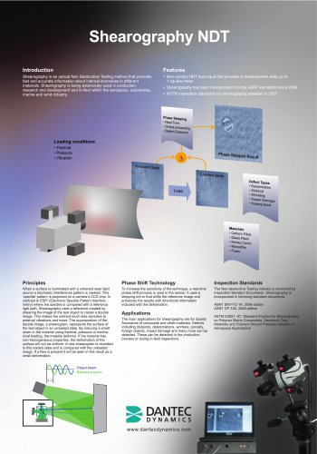 Shearography NDT
1 Page
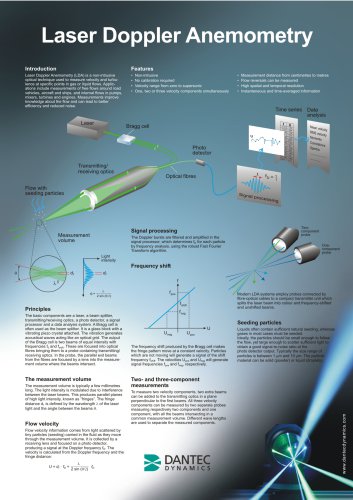 Laser Doppler Anemometry
1 Page